Update See sortvis.org for many more visualisations!
A couple of years ago, I blogged about a technique I came up with for statically visualising sorting algorithms during a somewhat Scotch-fueled night of idle hacking. A recent day of poking at the Python codebase gave me an excuse to revisit the post and brush off the bit of code that underpins it. I've wanted to take a closer look at timsort - Tim Peters' wonderful sorting implementation for Python - for a while now. In the previous post I made a big deal about the fact that many attributes of sorting algorithms are easier to see in my static visualisations than in traditional animated equivalents. So, I thought it would be fun to see if one could get to grips with a real-world algorithm like timsort by visualising it. The fruit of my labour can be found below - if this kind of thing turns your crank, read on.
Before you go on, you might first want to take a look at the original post for an explanation of how the diagrams are constructed and some related caveats.
Inspecting timsort
The first step was to get hold of the progressive sorting data I needed for the visualisation. The way timsort is implemented has two properties that helped here - firstly, it's largely in-place, and secondly, when interrupted by an exception in the __cmp__ method of one of the elements it is sorting, it leaves the array partially sorted. The pleasant result is that I could get all the data I needed in pure Python, without instrumenting the interpreter source. A link to the code is at the bottom of this post.
A first guess at the algorithm
The first thing I did was to see if I could get a feel for timsort straight from the visualisation, without looking at the implementation (yes, I'm cheating slightly, since I already had an idea of what I would see). Here's timsort sorting a shuffled array of 64 elements:
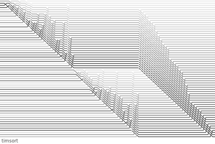
It's immediately clear that timsort has divided the data up into two blocks of 32 elements. The blocks are pre-sorted in turn (the first two "triangles" of activity, reading from left to right), before being merged together in the final step (the cross-hatch pattern at the right of the diagram). Looking closer, it's even possible to tell that the pre-sorting seems to be using insertion sort - compare the distinctive triangular pattern here with the insertion sort visualisation in the previous post. We can confirm this by taking the same data, and running it through an insertion sort visualisation. Here's the first block of 32 elements sorted by insertion sort:
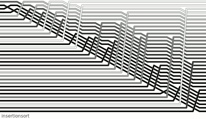
As you can see, this sorting sequence is identical to the one in the upper-left part of the timsort diagram. A similar bit of hackery would show that the final merge is done with mergesort. Ok, so at this point, we can take a stab at a broad outline of the timsort algoritm: break the data up into blocks, pre-sort those blocks using insertion sort, and then merge the blocks together using mergesort.
This is pretty good going for quick inspection of a single diagram.
What's actually happening
Flicking to the cheat sheet, we can see that this guess is almost right. The business-end of timsort is a mergesort that operates on runs of pre-sorted elements. A minimum run length minrun is chosen to make sure the final merges are as balanced as possible - for 64 elements, minrun happens to be 32. Before the merges begin, a single pass is made through the data to detect pre-existing runs of sorted elements. Descending runs are handled by simply reversing them in place. If the resultant run length is less than minrun, it is boosted to minrun using insertion sort. On a shuffled array with no significant pre-existing runs, this process looks exactly like our guess above: pre-sorting blocks of minrun elements using insertion sort, before merging with merge sort.
We can see a bit more detail by giving timsort the type of data it excels at - a partially sorted array:
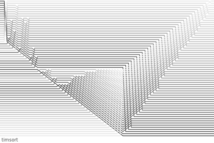
Now, looking at the marked progression from left to right:
- 1) timsort finds a descending run, and reverses the run in-place. This is done directly on the array of pointers, so seems "instant" from our vantage point.
- 2) The run is now boosted to length minrun using insertion sort.
- 3) No run is detected at the beginning of the next block, and insertion sort is used to sort the entire block. Note that the sorted elements at the bottom of this block are not treated specially - timsort doesn't detect runs that start in the middle of blocks being boosted to minrun.
- 4) Finally, mergesort is used to merge the runs.
Of course, there's a lot that's not covered here: merge order, stability, the secondary memory requirements of the algorithm, and so forth. Maybe I'll get to some of these in a follow-up post. That said, I think this is still quite a reasonable high-level pictorial guide to timsort.
I relied heavily on Uncle Tim's own description of the algorithm in writing this post - if you're interested in timsort, this document is definitely mandatory reading.
The Code
I've brushed up the code I included in my previous post and put it on github. You can check it out like so:
git clone git://github.com/cortesi/sortvis.git