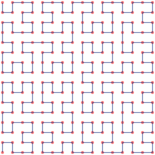
The Hilbert curve is a remarkable construct in many ways, but the thing that makes it useful in computer science is the fact that it has good clustering properties. If we take a curve like the one above and straighten it out, points that are close together in the two-dimensional layout will also tend to be close together in the linear sequence. I say "tend to be", because we can never get this perfectly right - we can show that any curve of this type will have some points that are close to each other spatially but far from each other on the curve. It turns out, however, that the clustering behaviour of the Hilbert curve is pretty much as good as we can currently get. For one example of how this property can be useful, imagine that we have a database with two indexes - X and Y. We know that we will be doing frequent queries on those indexes, asking for records where X and Y fall within specified ranges. We can visualise this as retrieving rectangular regions from a two-dimensional space. Given this scenario, how can we lay out the records on disk to minimise disk access? Information on disk is stored sequentially, so what we want is a layout that maximises the likelihood that records in any given rectangular region will also be adjacent on disk. In other words, what we want is a way to order our two-dimensional space of records so that records close to each other in two dimensions also tend to be close to each other in the sequential order. This is exactly the outstanding property of the Hilbert curve, so one solution is to store our records on disk in Hilbert order.
Visualising the Hilbert curve: A first stab
I've long felt that the usual visualisation of the Hilbert curve - like the one shown at the top of this post - doesn't really do its clustering properties justice. The lines-and-vertices approach demonstrates how to construct the curve very nicely, but it doesn't give us any intuitive feel for how close points on the curve are to each other on the plane. In the remainder of this post, I take a stab at visualising the Hilbert curve as the great mathematician in the sky intended - completely covering the plane, and with each pixel visually encoding its proximity to its neighbours along the curve.
One way to proceed would be to find a way to assign a colour every pixel in a Hilbert-order traversal of a square image. Imagine the RGB colour space as a cube where each colour is uniquely identified by a set of (r, g, b) co-ordinates. Here's one with 20 colours to a side:
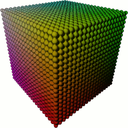
We'll use a somewhat larger colour cube - 256 colours to a side, giving us 16 777 216 unique colours. This colour cube is familiar to pretty much everyone, since it's precisely the colour space we use when we specify HTML-style #rrggbb colours. We can project the RGB colour cube at 1:1 resolution onto a square with 4096 pixels to a side - this exactly matches a Hilbert curve of order 12. Now we need a method for traversing the colours in the colour cube. One trivial way to do this is to simply snake through all the points in the cube. In two dimensions, it would look like this:
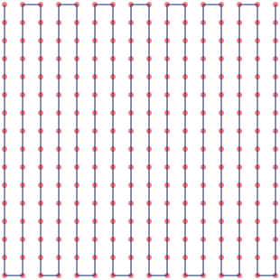
This generalises to 3 or more dimensions easily - just imagine "stacking" plates of two-dimensional traversals in such a way that one plate's end point is adjacent to the next plate's starting point. For want of a better term, I've called this Zigzag order. When we project a Zigzag traversal of the RGB colourspace onto a Hilbert-order traversal of the plane, we get this:
That's... ugly. You can vaguely make out the shape of the Hilbert curve by dividing the image into quadrants, and traversing them in the order in which they blend into each other. But there's a problem - if we traverse the RGB colour space in Zigzag order, many colours that are close to each other in 3d space - and therefore visually similar - are quite far from each other in our traversal order. This is what causes the blotchy artifacts in the image above. What we really want is a traversal of the RGB colour space that is as smooth and continuous as possible - meaning that colours that are close to each other in the cube are also as close as possible to each other in the traversal order. Wait a minute... that sounds familiar, doesn't it?
Drawing the Hilbert curve in N dimensions
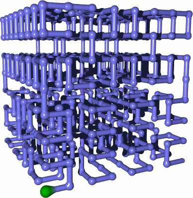
What we really want is a 3d Hilbert curve traversal of the RGB colour cube. This would mean that our colour clustering - making sure that similar colours are as close as possible to each other in the sequence - would be close to optimal. We should then see the clustering properties of the 2d Hilbert curve as patches of similar colour. So, does a 3d analogue to the Hilbert curve exist? Sure it does - here's a somewhat befuddling picture of an example rendered with POV-Ray:
We can do even better than 3 dimensions, though, by generalising the Hilbert curve to N dimensions. Concretely, we would like to find a way to translate an offset along the N-dimensional Hilbert curve to co-ordinates, and vice-versa. The algorithms to do this are somewhat tricky, but are well known and widely described. A particularly nice exposition can be found in the paper "Compact Hilbert Indices" by Chris Hamilton. This section is based on Hamilton's version of the classic algorithm first devised by A. R. Butz in the 1970s (though, see comments in my code for corrections to some minor errors in the paper that may trip up implementers).
We start with a slight detour - the surprising connection between the Hilbert curve and Gray codes. Recall that Gray codes are a way to traverse all numbers of a given bit width in such a way that only one bit differs from each value to the next. Here, for example, are the 2-bit and 3-bit Gray codes:
2-bit
0, 0
0, 1
1, 1
1, 0
3-bit
0, 0, 0
0, 0, 1
0, 1, 1
0, 1, 0
1, 1, 0
1, 1, 1
1, 0, 1
1, 0, 0
Now, watch what happens when we treat each set of bits in the N-bit Gray code as co-ordinates in N-dimensional space (with X being the rightmost bit), and draw the resulting curves:
| 2-bit | 3-bit |
|---|---|

|
|
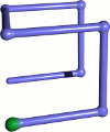
Voila, the Order 1 Hilbert curves in 2 and 3 dimensions! A bit of pondering shows that this generalises to any dimension - if we have a hypercube with dimensions 1x1x1..., the Gray code will traverse all the vertices of the cube by changing only one dimension at a time. Specifically, we can say that the N-bit Gray code is a Hilbert order traversal of the vertices of an N-dimensional hypercube. Effectively, this means that we can now draw the Order 1 Hilbert curve for any dimension - so let's refresh our memories of how the Order 1 curve relates to the higher orders.
| O1 | O2 | O3 |
|---|---|---|

|
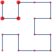
|
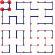
|
Notice that as we move from one order to the next, we replace each vertex with a sub-curve that has the same shape as the O1 traversal. I've marked one path through this recursive process in the images above, showing the subcurve for the upper-left vertex in every step of the recursion. At every step, we also need to transform the subcurve through rotation and reflection to make sure that its start matches the end of the previous subcurve, and its end matches the beginning of the next subcurve. This process generalises trivially to N dimensions. Since the O1 curve is just a Gray code traversal of the N-dimensional cube, we can think of the Order M Hilbert curve as a collection of hypercubes nested M deep.
Now, let's see if we can use this construction process to figure out the co-ordinates of a point, given the offset along the Hilbert curve. We'll ignore the rotations and reflections for the moment. We start with the O1 curve of dimension N, and the N most significant bits of the offset. By checking which vertex of the hypercube this maps to, we can peel off the most significant bit of each co-ordinate. For example, if we wanted to locate offset 63 in the 2-dimensional Order 3 curve (the upper-left corner), our first two bits would be (1, 1). This is the fourth point in the Gray code traversal of the hypercube, which gives us the upper-left quadrant of the O1 cube. We now know that the most significant bit of our X co-ordinate is 0, and the most significant bit of our Y co-ordinate is 1. Doing the same thing for the matching sub-hypercube in the O2 curve will give us the next bit, and we can drill down through the hypercubes in this way peeling off one bit of each co-ordinate, until we have all M bits. This process also works in reverse - if we start with a set of co-ordinates, we can drill down through the hypercubes, determining N bits of the curve offset at every step. So, generally, at every step of the Gray code recursion we get a nested hypercube of dimension N, and N bits of co-ordinate or offset information. Finally, we need to deal with the rotations and reflections required to make the heads and tails of the Gray code subcurves match up. We'll need to perform this transformation at every step, before we extract our information bits. All we need is a way to rotate and reflect a given hypercube to make its beginning and end match up with its position on the curve. The transform required turns out to map to a simple set of bit operations described in Section 2.3.1 of Hamilton's paper.
And that's it - using this general process, we can now calculate co-ordinates or offsets for points on an N-dimensional Hilbert curve. Hopefully, I've managed to give some intuition for how this algorithm works, but I've glossed over pretty much all the details. See the original paper or the code I'm publishing for specifics. I should also note in passing that this is just one way to draw the Hilbert curve - at higher dimensions there are many, many different well-formed Hilbert curves.
A portrait of the Hilbert curve as a young fruit salad
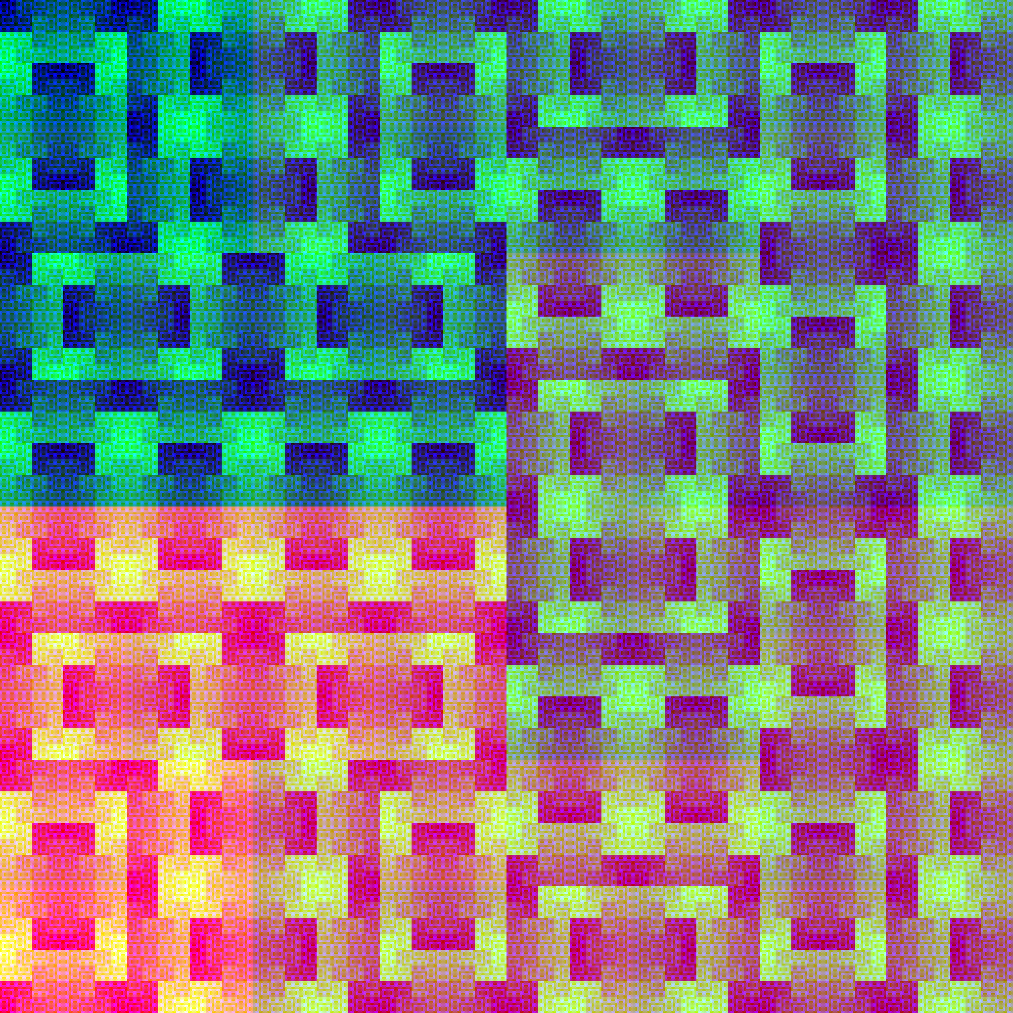
At last we are in a position to traverse the 3-dimensional RGB cube in Hilbert order, and have another stab at visualising the 2d Hilbert curve.
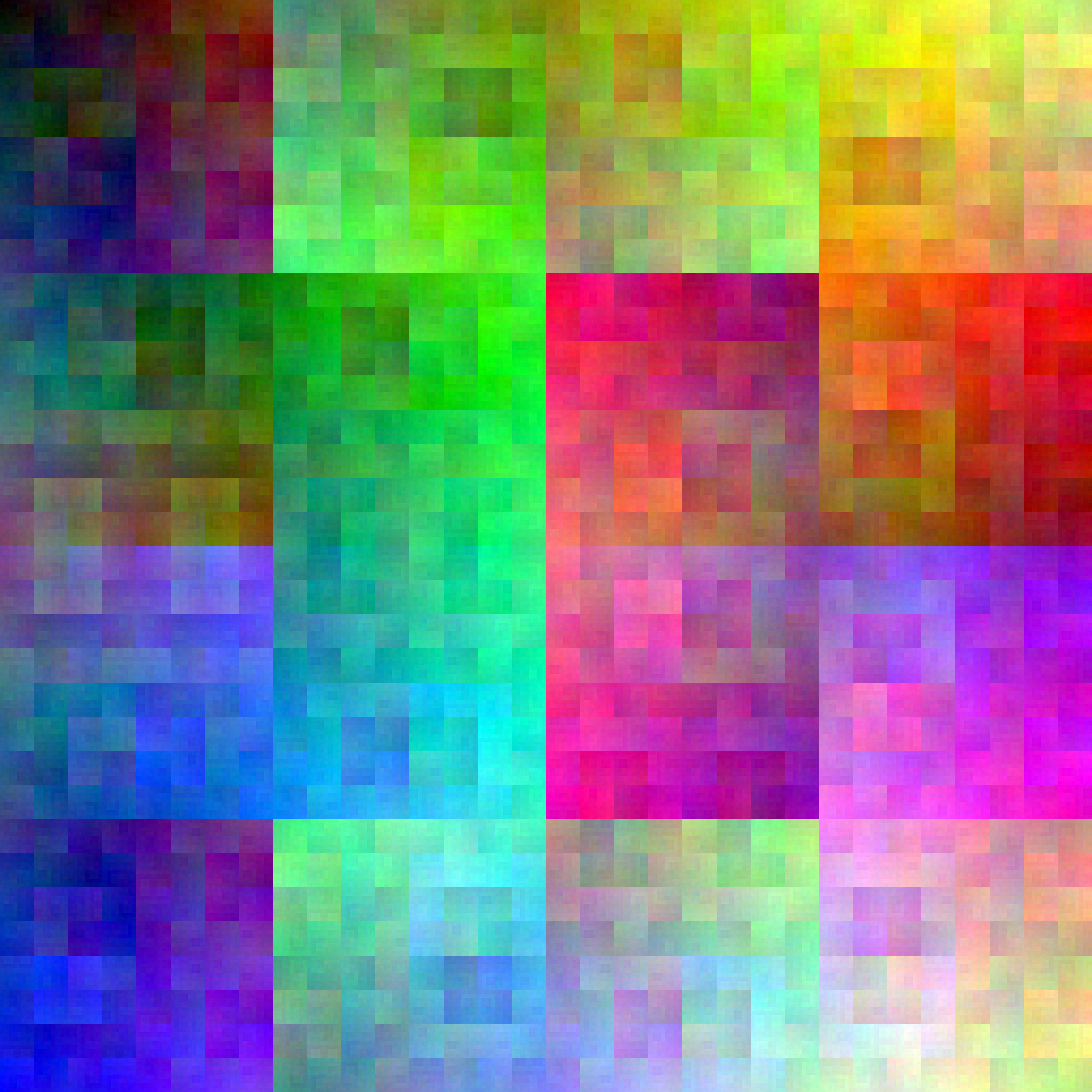
Ladies and gentlemen, I present a Hilbert curve traversal of the three-dimensional RGB colour space, projected onto a two-dimensional Hilbert curve covering the plane. I think it's absolutely damn beautiful. Like some weird piece of abstract art - a Kandinsky or perhaps a Pollock - the more you look at this image, the more structure you see. If you divide it into quadrants, and sub-quadrants, and sub-sub-quadrants, you can trace the path of the Hilbert curve at every level of recursion by following the flow of colours (use the 2d Hilbert curves elsewhere in this post for reference if you're having trouble). If you're looking at the full-size image, this works even at very large magnifications, until the human ability to perceive colour differences starts to fail. Incredibly, this image contains exactly the same set of colours as the unattractive Zigzag visualisation at the start of the post - the only difference is the way the colours are arranged. This is so remarkable that you might want to verify this yourself using the colour analysis functionality of your favourite image editor (make sure you use the full-size images for best effect). We've also achieved the goal we set out with - the clustering properties of the 2d Hilbert curve are directly visible as patches of similar colour.
By the way - if Hilbert curves float your boat, you may also be interested in a previous post of mine, in which I visualise an IP geolocation database with Hilbert curves.
The code
git clone git://github.com/cortesi/scurve.gitI've released the code used to render the images in this article as a Python project called scurve (for space-filling curve). This project aims to be collection of clear implementations of algorithms related to space filling curves, together with a set of tools for visualising them. If you're interested in this kind of thing keep an eye on the project - I plan to add more interesting goodies in the next few weeks.